Is it possible to accidentally solve the wrong mathematical problem?

Using computers to solve mathematical problems approximately is something that happens everyday. Our weather forecasters, the people who design our buildings and even your calculator all use clever computer programs to find approximate answers to difficult mathematical problems.

But does it always work?

As an example, let’s look at something called advection, which is (more or less) just a fancy word for “floating along with the water”. When you throw a stick into a flowing river, the stick is advected downstream. All sorts of things can be advected; sticks, Prime Ministers, heat and salt to name just a few.

In the real world we usually expect things to spread out as they are carried along by the water; a process called diffusion. It’s important that our models include the right amount of diffusion, otherwise they lead to unrealistic predictions. To explore the difficulties in this we need some maths, in particular we need the one-dimensional diffusive advection equation:

$\frac{\partial\phi}{\partial t}+u\frac{\partial\phi}{\partial x}=\kappa\frac{\partial^2\phi}{\partial x^2},$

in which $\phi$ is the quantity being advected in the $x$ -direction with speed $u$ and $\kappa$ is the rate of diffusion. Let’s call this “equation 1”.

If you’ve studied some maths, you’re probably thinking “Aha! Just set $\kappa$ to the right value and we’re fine”. Unfortunately it’s not as simple as that.

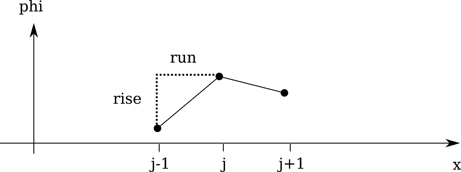
When we use a computer to solve equations like this we need to discretise the equations. That is, we break the equation up into lots of small chunks and write a computer program to solve the large number of simpler equations. This picture shows a function phi ( $\phi$ ) that has been discretised. The derivative of $\phi$ with respect to $x$ can be approximated by the rise over the run.

Now the derivative can be approximated like this:

$\frac{\partial \phi}{\partial x} \approx \frac{\phi_{j}-\phi_{j-1}}{x_{j}-x_{j-1}} \equiv \frac{rise}{run}.$

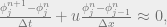
To illistrate how this can lead to solving the wrong problem, I’m going to set $\kappa$ to be zero and see what happens. Approximating the derivatives with tangents (rise over run from high-school maths) gives this equation:

$\frac{\phi^{n+1}_{j}-\phi^{n}_{j}}{\Delta t} + u \frac{\phi^{n}_{j}-\phi^{n}_{j-1}}{\Delta x} \approx 0,$

where the superscripts refer to the $n$ th or the $(n+1)$ th time step.

After a bit of rearranging we get a simple equation for $\phi$ at time $n+1$ and at the $j$ th point along $x$ :

$\phi^{n+1}_{j} = \frac{u \Delta t}{\Delta x} \left(\phi_{j-1}^{n} -\phi_{j}^{n}\right) + \phi^{n}_{j}$

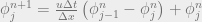
Let’s call this “equation 2”.

Now we can use a computer to solve this equation, and even to make a movie of the solution.

But what happened here? Didn’t we set $\kappa$ to be zero? Why is there diffusion?

To answer these questions we need to dive into some more maths. In particular Taylor Series. Using Taylor Series to represent the different values of $\phi$ we get:

$\phi^{n+1}_{j} = \phi^{n}_{j} + \Delta t \frac{\partial \phi}{\partial t} + \frac{\Delta t^{2}}{2}\frac{\partial^2 \phi}{\partial t^{2}}+ \dots$
$\phi^{n}_{j-1} = \phi^{n}_{j} - \Delta x \frac{\partial \phi}{\partial x} + \frac{\Delta x^{2}}{2}\frac{\partial^{2} \phi}{\partial x^{2}} - \dots$

If we substitute these expressions back into equation 2 then we get:

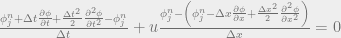
$\frac{\phi^{n}_{j} + \Delta t \frac{\partial \phi}{\partial t} + \frac{\Delta t^{2}}{2}\frac{\partial^2 \phi}{\partial t^{2}} - \phi^{n}_{j}}{\Delta t} + u \frac{\phi^{n}_{j}-\left(\phi^{n}_{j} - \Delta x \frac{\partial \phi}{\partial x} + \frac{\Delta x^{2}}{2}\frac{\partial^{2} \phi}{\partial x^{2}} \right)}{\Delta x} = 0$

A bit of rearranging and cancelling gives the following equation:
$\frac{\partial \phi}{\partial t} + u \frac{\partial \phi}{\partial x} =-\frac{u^2 \Delta t}{2} \frac{\partial^2 \phi}{\partial x^2} + \frac{u \Delta x}{2}\frac{\partial^2 \phi}{\partial x^2} = \left(\frac{u \Delta x}{2} - \frac{u^2 \Delta t}{2}\right) \frac{\partial^2 \phi}{\partial x^{2}},$

which looks a lot like the original diffusive advection equation (equation 1 in case you’ve forgotten) with
$\kappa = \frac{u \Delta x}{2} - \frac{u^2 \Delta t}{2}.$

It’s possible to “tune” this very simple model to remove diffusion by setting
$u \Delta t = \Delta x.$

As you can see in the next video.

But this brings us uncomfortably close to the limit of the Courant-Friedrichs-Lewy condition for stability:
$u \Delta t \leq \Delta x.$

Even this solution doesn’t always help. It is often impossible to tune more complex models in this way, especially global models for weather and climate, because the grid size is not uniform across the globe. If we increase the time step (or decrease the step in $x$ ) by just 3%, then the numerical scheme becomes unstable.

If $\phi$ represents the concentration of salt, how do we interpret a negative concentration?

There are lots of clever methods that have been devised to numerically model advection, but so far, none of them are perfect. The methods that give the most realistic answers take a lot of computer power to implement and the ones that can easily be implemented often give unrealistic results in all but the simplest of situations.

All of this means that the answer is yes; it is possible to solve the wrong equation by mistake. This has profound implications for weather and climate models and is one of the reasons that mathematics is still an active area of research.

Thanks to Liam and Renske for leading a discussion about numerical schemes for advection during a recent group meeting.

Other interesting and related things to look at:

Prather, M. J., Numerical advection by conservation of second-order moments, J. Geophys. Res., 91, 6671-6681, 1986.

This is Prather’s seminal paper describing the use of quadratic interpolation between grid boxes to limit numerical diffusion. “A comparison of the capabilities of different algorithms shows that each scheme has its advantages and that no one method is most advantageous under all conditions.”

This presentation gives a good (if somewhat technical) overview of the numerical advection problem.

Edward Doddridge

Physical Oceanographer

Is it possible to accidentally solve the wrong mathematical problem?

Other interesting and related things to look at:

Leave a Reply Cancel reply

Other interesting and related things to look at:

Share this:

Like this:

Leave a Reply Cancel reply